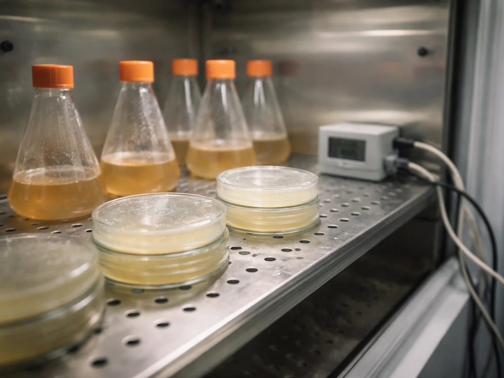
When a textbook or worksheet says 'a bacteria culture is known to grow at a rate of…', it is giving you the specific growth rate (µ), a single number that tells you how fast the population multiplies per unit of time. Growthcurver: an R package for obtaining interpretable metrics from microbial growth curves (Sprouffske & Wagner, BMC Bioinformatics 2016) notes that Tools and example datasets for classroom exercises: the R package 'growthcurver' (Sprouffske & Wagner 2016, BMC Bioinformatics) fits logistic models to OD growth curves and provides interpretable parameters (r, K, N0); authors and associated GitHub/repositories include example data useful for teaching curve fitting and model comparison. From that one number you can calculate the doubling time, predict population size at any future moment, and understand what environmental conditions are driving or limiting that growth. This article walks through all of that, the definitions, the math, the measurements, the models, and the real-world context, for students, educators, and anyone who wants to understand what that deceptively simple phrase actually means.
a bacteria culture is known to grow at a rate: definitions & time

What those key terms actually mean
Before doing any math, it helps to have clean definitions for the terms that keep appearing in growth problems. They are often used loosely in introductory materials, and that looseness causes real confusion when students try to set up equations.
| Term | Symbol | Definition | Typical Units |
|---|---|---|---|
| Specific growth rate | µ (also written k) | Rate of increase in cell number per cell per unit time: µ = (1/N) dN/dt = d(ln N)/dt | h⁻¹ or min⁻¹ |
| Growth constant | µ or k | Same quantity as specific growth rate; 'constant' implies it is fixed under a given set of conditions | h⁻¹ |
| Doubling (generation) time | t_d or g | Time required for the population to double: t_d = ln(2) / µ | hours or minutes |
| Death rate | k_d | Rate at which cells lose viability per unit time; net growth = µ − k_d | h⁻¹ |
| Carrying capacity | K | Maximum population density a given environment can sustain; growth slows to zero as N → K | cells·mL⁻¹ or OD units |
The specific growth rate µ is the most important of these. It is an intrinsic, per-capita rate: think of it as each individual cell's contribution to population change. A µ of 1.0 h⁻¹ does not mean the culture grows by 1 cell per hour, it means the population increases by 100% of itself every hour when growth is exponential. Carrying capacity is at the other end of the story: it represents the ceiling that resource limitation and waste accumulation impose on that growth, which is why batch cultures always slow down and stop.
How growth rate and doubling time relate (with quick conversions)
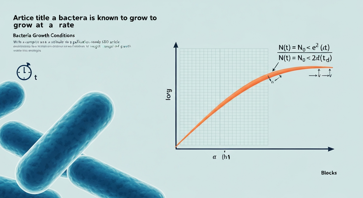
The relationship between µ and doubling time td is one of the most commonly tested conversions in microbiology courses, and it is beautifully simple. If N doubles, then N(td) = 2·N₀. Plugging into the exponential equation N(t) = N₀ · e^(µt) gives 2 = e^(µ·t_d), so taking the natural log of both sides:
- t_d = ln(2) / µ ≈ 0.693 / µ
- µ = ln(2) / td ≈ 0.693 / td
- Units must match: if µ is in h⁻¹, then td is in hours; if µ is in min⁻¹, then td is in minutes
A worked example helps cement this. Suppose µ = 0.693 h⁻¹. Then t_d = 0.693 / 0.693 = 1.0 h exactly, the culture doubles once per hour. Now flip it: if a textbook tells you E. coli doubles every 20 minutes under optimal lab conditions, then µ = 0.693 / 20 min = 0.0347 min⁻¹, or equivalently 2.08 h⁻¹. These two forms of the same information appear interchangeably in problems, so being comfortable converting in both directions is essential.
| Given µ (h⁻¹) | Doubling time t_d | Given t_d | Calculated µ (h⁻¹) |
|---|---|---|---|
| 0.693 | 1.0 h | 20 min (0.33 h) | 2.08 |
| 0.347 | 2.0 h | 1 h | 0.693 |
| 0.116 | 6.0 h | 3 h | 0.231 |
| 0.028 | 24.7 h | 12 h | 0.0578 |
Predicting population changes: the exponential growth equation with worked examples
During the log (exponential) phase, bacterial population growth follows: N(t) = N₀ · e^(µt), where N₀ is the starting cell number, N(t) is the population at time t, µ is the specific growth rate, and t is elapsed time in the same units as µ. An equivalent form using doubling time is N(t) = N₀ · 2^(t / t_d), which many students find more intuitive because it directly counts the number of doublings.
Worked example 1: predicting final population
A bacteria culture is known to grow at a rate of µ = 0.35 h⁻¹. The starting population is N₀ = 1 × 10⁴ cells·mL⁻¹. How many cells·mL⁻¹ are present after 8 hours?
- Write the equation: N(t) = N₀ · e^(µt)
- Substitute values: N(8) = 1×10⁴ · e^(0.35 × 8)
- Calculate the exponent: 0.35 × 8 = 2.80
- Find e^2.80 ≈ 16.44
- Multiply: N(8) ≈ 1×10⁴ × 16.44 ≈ 1.64 × 10⁵ cells·mL⁻¹
Worked example 2: finding µ from two data points
You measure OD600 = 0.10 at t = 0 h and OD600 = 0.55 at t = 5 h during the exponential phase. What is µ? During exponential growth ln(N) is linear in time, so µ = (ln N₂ − ln N₁) / (t₂ − t₁) = (ln 0.55 − ln 0.10) / (5 − 0) = (−0.598 − (−2.303)) / 5 = 1.705 / 5 = 0.341 h⁻¹. The doubling time is then t_d = 0.693 / 0.341 ≈ 2.03 h.
Classroom practice problem
A culture starts with 5 × 10³ cells·mL⁻¹ and has a doubling time of 45 minutes. How many cells·mL⁻¹ are present after 3 hours? Answer: td = 45 min = 0.75 h; number of doublings = 3 / 0.75 = 4; N(3 h) = 5×10³ × 2⁴ = 5×10³ × 16 = 8 × 10⁴ cells·mL⁻¹. Student activity sheets exploring similar growth scenarios can be found in related materials on this site, and simulated environment exercises model these same calculations under controlled virtual conditions.
How to actually measure growth in the lab
There is an important gap between the clean equations above and real experimental data. Measuring bacterial population size requires choosing a method, and every method has assumptions and failure modes that affect how you interpret the numbers. Here are the four most common approaches used in educational and research settings.
Optical density at 600 nm (OD600)
OD600 is the fastest and most common real-time measurement. The spectrophotometer shines light at about 600 nm through the culture; bacteria scatter that light, and the instrument reads a reduction in transmitted signal as 'absorbance'. The key point: OD600 measures turbidity (light scattering by cells), not true absorbance by a chromophore. It correlates with total biomass (live plus dead cells), not just viable cells. For a standard 1-cm path cuvette, the measurement is roughly linear only up to OD600 ≈ 0.6–0.8. Above that, multiple scattering and detector nonlinearity mean the reading underestimates true cell density, so you must dilute the culture and multiply back. For E. coli in mid-log phase, a commonly cited textbook conversion is approximately 6–8 × 10⁸ cells·mL⁻¹ per OD600 unit, but this varies enough between strains, instruments, and media that you should always build your own calibration curve rather than borrowing someone else's. BioNumbers (database), OD600 / cells·mL conversions and related entries (E. coli) summarizes measured ranges (e.g., ≈6–8×10^8 cells·mL⁻¹ per OD600 in mid‑log E. coli) and cites the primary calibration data; consult it when choosing or reporting a conversion BioNumbers (database) — OD600 / cells·mL conversions and related entries (E. coli).
Colony-forming units per mL (CFU·mL⁻¹)
Plate counting gives you viable, culturable cells specifically. You serially dilute the culture, spread known volumes on agar plates, incubate, and count colonies. The method assumes one colony arises from one viable cell unit, but clumping, filamentous morphology, and the 'viable but non-culturable' (VBNC) state all violate that assumption, leading to underestimates. Standard practice is to count only plates in the 30–300 colony range where Poisson counting statistics are reasonably well-behaved. Outside that window, results are either too imprecise (fewer than 30) or too crowded to count accurately (more than 300).
Direct microscopic counting
A haemocytometer or Petroff-Hausser counting chamber gives a total cell count (live and dead) by directly visualising cells under a microscope. It is inexpensive and requires no culturing, but it is slow, prone to observer error, and cannot distinguish live from dead cells without viability stains. It works best for dense cultures and relatively large cells.
Flow cytometry and other methods
Flow cytometry can count cells rapidly while also reporting physiological state through fluorescent dyes that distinguish live, dead, and VBNC populations. It is powerful but expensive, making it less common in teaching labs. ATP-bioluminescence assays serve as a metabolic proxy (more ATP roughly equals more active biomass) and are widely used in food safety testing. Dry weight measurement is the gold standard for biomass in bioprocess engineering but requires large sample volumes and is too slow for routine growth curves.
| Method | What it measures | Detects VBNC? | Linear range / limit | Best for |
|---|---|---|---|---|
| OD600 | Turbidity (total biomass proxy) | Yes (all cells scatter light) | OD 0–0.8 in 1-cm cuvette | Real-time, fast growth curves |
| CFU·mL⁻¹ plate count | Viable, culturable cells | No (VBNC excluded) | 30–300 colonies per plate | Viability, food safety testing |
| Direct microscopy | Total cells (live + dead) | Yes | ~10⁶–10⁸ cells·mL⁻¹ | Morphology, quick total counts |
| Flow cytometry | Individual cells + physiology | Yes (with dyes) | Wide dynamic range | Research, live/dead discrimination |
| ATP assay | Metabolic activity proxy | Partially | Instrument-dependent | Food safety, rapid screening |
| Dry weight | Total biomass mass | Yes (all biomass) | Requires large volume (>50 mL) | Bioprocess engineering, bulk biomass |
The four phases of bacterial growth and what µ means in each
A standard batch growth curve has four phases, and the specific growth rate µ behaves differently in each. Understanding this prevents a very common student mistake: assuming the rate you calculated from one time window applies to the entire experiment.
Lag phase
When bacteria are inoculated into fresh medium, there is a period before net cell division begins. Cells are metabolically active, synthesising enzymes, adjusting to the new environment, repairing any damage from the previous growth state, but the population count barely changes. Effective µ ≈ 0 during this phase. The length of lag depends on the size and physiological state of the inoculum, the difference between the old and new medium, and the temperature shift involved. A culture transferred from a similar environment into the same medium at the same temperature will have a shorter lag than one shifted from 4°C into a different medium.
Exponential (log) phase
This is where balanced growth occurs: cells are dividing at a constant, maximum rate for the given conditions, and µ is at its highest value. Every cellular component (DNA, RNA, protein) doubles in concert. The population plot on a semi-log scale (log y-axis versus linear time) is a straight line during this phase, and the slope of that line equals µ. This is the phase targeted when a problem says 'a bacteria culture is known to grow at a rate of…', the stated rate almost always refers to log-phase growth. The worked examples above are all log-phase calculations.
Stationary phase
Growth slows and then stops as nutrient concentration falls, toxic metabolic by-products (organic acids, CO₂) accumulate, and the population approaches the carrying capacity K of the vessel. The net growth rate reaches zero: cell division and cell death are occurring at roughly equal rates, so the viable count plateaus. µnet ≈ 0, but both µ and kd are greater than zero. Bacteria in this phase often activate stress-response pathways and can enter the VBNC state, which is why CFU counts can diverge from OD600 readings at this stage.
Death phase
Resources are exhausted and toxic products dominate. The death rate k_d exceeds µ, so viable cell numbers fall, often exponentially at first. OD600 may remain elevated even as CFU counts plummet because dead cell debris still scatters light. This phase is particularly relevant for food safety: a product that looks turbid (high OD) is not necessarily full of living bacteria, and a culture that looks clear is not necessarily sterile.
Environmental factors that push µ up or down
The specific growth rate µ is not a fixed property of a bacterial species, it is the species's response to its current environment. The same E. coli strain that achieves µ = 2.0 h⁻¹ in a warm, well-aerated broth may struggle to reach µ = 0.1 h⁻¹ in a cooler, oxygen-depleted setting. Here is how each major factor contributes.
Temperature
Temperature is the single most powerful environmental lever on growth rate. Each bacterial species has a minimum, optimum, and maximum temperature for growth. Between the minimum and optimum, µ roughly doubles for every 10°C rise (a rule of thumb described by the Q₁₀ concept). Above the optimum, heat begins to denature enzymes and membrane lipids faster than the cell can compensate, and µ drops sharply to zero. This is why refrigeration (around 4°C) slows food spoilage, it pushes most mesophilic pathogens below their growth minimum, and why cooking kills bacteria by exceeding their thermal maximum.
pH
Most human-associated pathogens (mesophiles) grow optimally between pH 6.5 and 7.5. Extremes of pH denature proteins and disrupt membrane function. Acidic environments (pH < 4.6) are routinely used in food preservation, pickled vegetables, fermented dairy, vinegar-based condiments. The stomach's acidic environment (pH 1.5–3.5) is a major innate barrier to ingested pathogens. Certain bacteria (acidophiles) have evolved proton pumps and acid-resistant membrane compositions that allow growth at very low pH, which is why some spoilage organisms survive in acidic juices.
Oxygen availability
Bacteria are classified by their oxygen requirements: obligate aerobes (require O₂), obligate anaerobes (killed by O₂), facultative anaerobes (grow with or without O₂, but faster with it), microaerophiles (require low O₂), and aerotolerant anaerobes (tolerate O₂ but do not use it). Growth rate is directly tied to which respiratory or fermentative pathway is available. Agitation of liquid cultures (shaking flasks, stirred bioreactors) improves oxygen mass transfer and consistently raises µ for aerobes by preventing oxygen depletion, a factor that any experimental or simulated growth model needs to account for.
Moisture and water activity
Bacteria need water for all biochemical reactions, but the relevant metric is water activity (aw), not total water content. Pure water has aw = 1.0; most bacteria require aw > 0.91 for growth. Drying, salting, and sugar-curing foods reduce aw, which is why jerky, jam, and heavily salted fish resist spoilage without refrigeration. When a_w falls below the organism's minimum, µ drops to zero and the culture enters dormancy rather than growing.
Nutrients and substrate concentration
Growth rate depends on the availability of carbon, nitrogen, phosphorus, sulfur, and trace minerals. At high nutrient concentrations, µ reaches its ceiling µ_max. As a limiting nutrient is depleted, µ falls. This is precisely the relationship described by the Monod model (see the next section). In a batch culture, depletion of the limiting nutrient is the primary driver of the transition from exponential to stationary phase.
Inoculum size and carrying capacity
A larger inoculum reaches stationary phase faster simply because it starts closer to the carrying capacity K. It does not necessarily have a higher µ during log phase, but the log phase is shorter. Carrying capacity itself is set by the environment: the volume of the vessel, the initial nutrient concentration, and the tolerance limits of the organism for its own waste products. Understanding K is critical when interpreting growth curves from simulated environments, where researchers can manipulate K independently of µ to test model predictions.
Population models for classrooms and simulations
Three models dominate teaching and introductory research: the exponential model, the logistic model, and the Monod model. They are not competing, they describe different aspects of growth and are each appropriate in specific contexts.
Exponential model
Equation: dN/dt = µ · N, integrated to N(t) = N₀ · e^(µt). Assumptions: unlimited nutrients, constant µ, no death or inhibition. When to use: log-phase calculations, short-time predictions in food safety ('how many doublings in 4 hours?'), and initial conditions in all growth simulations. This model overestimates population size whenever resources become limiting, which is why it must be combined with a carrying capacity term for longer time horizons. Example parameters: N₀ = 1 × 10³ cells·mL⁻¹, µ = 0.5 h⁻¹.
Logistic (Verhulst) model
Equation: dX/dt = r · X · (1 − X/K), where r is the intrinsic growth rate (equivalent to µ at low density) and K is carrying capacity. The integrated form produces the familiar S-shaped (sigmoidal) curve that matches a complete batch growth curve from inoculation through stationary phase. Assumptions: growth rate decreases linearly as population approaches K; no explicit mechanism for the slowdown (nutrient depletion and waste accumulation are lumped into the K term). When to use: visualising all four growth phases in a single equation, classroom curve-fitting exercises, and comparing how different K values affect the shape of the growth curve. The R package growthcurver fits this model to OD600 data and returns interpretable parameters (r, K, N₀), making it a practical tool for student data-analysis exercises. Example parameters: r = 0.5 h⁻¹, K = 1 × 10⁹ cells·mL⁻¹, N₀ = 1 × 10³ cells·mL⁻¹.
Monod model
Equation: µ(S) = µmax · S / (Ks + S), where S is substrate (limiting nutrient) concentration, µmax is the maximum specific growth rate, and Ks is the half-saturation constant (the substrate concentration at which µ = ½ µmax). This is the biochemically grounded model for nutrient-limited growth, analogous in form to the Michaelis-Menten enzyme kinetics equation. When to use: understanding why µ falls as nutrients deplete, connecting substrate concentration to growth rate in continuous cultures or chemostats, and contextualising the Monod relationship in courses that include enzyme kinetics. Example parameters for E. coli on glucose: µmax ≈ 1.0–2.0 h⁻¹, K_s ≈ 0.01–0.1 g·L⁻¹ glucose (these vary by strain and conditions).
| Model | Core equation | Key parameters | Captures carrying capacity? | Best classroom use |
|---|---|---|---|---|
| Exponential | N(t) = N₀ · e^(µt) | µ, N₀ | No | Log-phase prediction, doubling-time problems |
| Logistic (Verhulst) | dX/dt = r·X·(1 − X/K) | r, K, N₀ | Yes (explicitly) | Full batch curve, curve-fitting exercises |
| Monod | µ = µ_max · S/(K_s + S) | µ_max, K_s, S | Indirectly (via S → 0) | Linking nutrient depletion to growth rate |
Growth rate in genetically modified bacteria: the conceptual picture
Engineered bacteria, those carrying a plasmid with an inserted gene, grow by the same mathematical principles as wild-type strains, but their effective µ under a given set of conditions may differ. For examples and practical protocols showing how bacteria are genetically modified to grow with new traits, see resources on bacteria are genetically modified to grow (internal ref 7fa46e72-f04e-48ad-a7e4-76aa34f32776). Maintaining and expressing a foreign gene costs metabolic energy (a 'metabolic burden'), which can reduce µ relative to the unmodified parent strain. For this reason, engineered strains are typically grown in selective media: an antibiotic resistance gene on the plasmid means that only bacteria that retain the plasmid can grow when the antibiotic is present. Bacteria that lose the plasmid (plasmid-free segregants) would otherwise out-compete the engineered strain because they no longer bear the metabolic cost. When interpreting growth curves from genetically modified cultures, the measured µ reflects the combined effect of the organism's baseline physiology, the metabolic burden of the plasmid, and the selection pressure imposed by the medium, a conceptually rich intersection of genetics, kinetics, and environmental control. For example, in lab protocols the bacteria containing the engineered plasmid would grow in antibiotic-containing selective media to ensure plasmid retention.
Real-world implications: food safety, hygiene, and experimental design
The numbers behind µ have direct, practical consequences. At µ = 0.5 h⁻¹ (a modest rate for a mesophilic pathogen at room temperature), a contamination event starting with just 100 cells reaches the commonly cited infectious dose of ~10⁶ cells in about 9.2 hours, well within a standard overnight period on a countertop. Refrigeration at 4°C does not eliminate growth; it lowers µ dramatically for most pathogens, extending that doubling time from 20–40 minutes to many hours or effectively stopping growth, but cold-tolerant organisms (psychrotrophs) still grow, which is why refrigerated foods eventually spoil. Knowing the doubling time also helps interpret food safety guidelines: the 'danger zone' (4°C to 60°C) is defined precisely because most pathogens have non-trivial µ values throughout that range.
In experimental design, failing to account for the growth phase of your inoculum introduces systematic error. Cells taken from stationary phase carry a physiological legacy (stress proteins, altered membrane composition, slower ribosomes) that extends lag time and may change apparent µ. The best practice for reproducible experiments is to use mid-log phase cells standardised to a known OD600, transferred into pre-warmed medium. This principle applies equally to virtual simulated growth environments, where initial conditions (phase, density, nutrient concentration) must be specified carefully for model outputs to be meaningful. For practical guidance on setting up and interpreting virtual experiments, see how do bacteria grow in a simulated environment.
Graphing growth data: conventions worth knowing
How you plot your data determines what you can see. There are two standard approaches, and both belong in any serious growth analysis. First, plot OD or cell count on an arithmetic y-axis versus time: this shows the full sigmoidal shape of the batch curve, making lag, log, stationary, and death phases visually obvious. Second, plot ln(OD) or log₁₀(cell count) on the y-axis versus time (semi-log plot): during exponential phase this produces a straight line, and the slope of that line directly equals µ (if using natural log) or µ/2.303 (if using log₁₀). Mark clearly on your graph which time window you used to fit the slope, because choosing a non-linear portion of the curve inflates or deflates µ. Both plots together tell the complete story, and presenting only one is a common oversight in student lab reports.
Common misconceptions and interpretation pitfalls
- Misconception: OD600 directly counts live cells. Reality: OD600 measures all light-scattering particles, including dead cells and debris. Use CFU counts or viability stains for live-cell-specific data.
- Misconception: a higher OD600 reading always means more cells. Reality: above OD ≈ 0.8 in a standard 1-cm cuvette, the reading saturates. Always dilute and back-calculate in this range.
- Misconception: µ is constant throughout an experiment. Reality: µ is only approximately constant during log phase. It is near zero in lag and stationary phases and negative (net) in death phase.
- Misconception: doubling time is the same as generation time. Reality: doubling time and generation time are synonymous in clonal bacterial cultures — they both describe the time for the population to double — but the terms are sometimes used differently in eukaryotic cell biology.
- Misconception: refrigeration kills bacteria. Reality: refrigeration slows or stops growth for most mesophiles but does not kill them; viable cells resume growth when returned to permissive temperatures.
- Misconception: a culture is sterile if the broth looks clear. Reality: low cell densities are invisible to the naked eye; a culture can contain up to ~10⁶–10⁷ cells·mL⁻¹ and still appear clear.
Biosafety and ethical considerations
Understanding growth kinetics is intellectually powerful, and that power comes with responsibility. Any work with live bacterial cultures, even non-pathogenic model organisms like K-12 E. coli, requires appropriate containment (at minimum Biosafety Level 1 procedures: lab coats, gloves, no mouth pipetting, proper decontamination before disposal). Cultures should never be discarded down the drain without autoclaving or chemical inactivation. For exercises involving genetically modified strains and plasmids, institutional biosafety committee (IBC) approval is required in most jurisdictions, even for commercially supplied educational kits. Calculating exponential growth rates for dangerous pathogens is a legitimate educational activity in the classroom; attempting to cultivate or experiment with such organisms outside an approved facility is not. These are not bureaucratic formalities, they reflect hard-learned lessons about the real-world consequences of uncontrolled microbial growth, the very phenomenon this article is about.
FAQ
What does the phrase "a bacteria culture is known to grow at a rate ..." mean in formal terms?
It means the population increases according to a defined specific (instantaneous) growth rate µ (also written k). Formally µ = (1/N)·dN/dt = d(ln N)/dt with units of inverse time (e.g., h⁻¹). During exponential (log) phase this gives N(t)=N0·e^{µt}. Saying a culture "grows at a rate 0.5 h⁻¹" implies that the natural‑log increase of the population is 0.5 per hour.
How is doubling (generation) time related to the growth rate?
Doubling time t_d is the time required for population size N to double. It relates to µ by t_d = ln(2)/µ ≈ 0.693/µ. Example: if µ = 0.693 h⁻¹ then t_d = 1.0 h (one doubling per hour). Conversely, µ = ln(2)/t_d.
What are the canonical mathematical models used to represent bacterial population change?
Key simple models useful in teaching: - Exponential (ideal, unlimited resources): N(t)=N0·e^{µt}. - Logistic (resource limitation/carrying capacity K): dN/dt = r·N·(1−N/K); yields an S‑shaped curve; useful to illustrate stationary phase. - Monod (substrate‑limited specific growth): µ(S)=µ_max·S/(K_s+S), where S is limiting substrate, µ_max is max specific rate, K_s is half‑saturation constant. Use exponential for short log‑phase windows, logistic to model saturation, and Monod to connect µ to nutrient concentration.
How do you extract µ from experimental data?
During the exponential (log) phase: - Measure a quantity proportional to biomass (e.g., OD600 or cell counts) vs time. - Plot ln(measure) versus time; the slope of the linear region equals µ. - Numerically: µ = [ln(N2) − ln(N1)]/(t2 − t1). Always report the time window used and units (h⁻¹ or min⁻¹).
What are common measurement methods and what do they report (strengths/limitations)?
Common classroom/bench methods: - OD600 (turbidity): quick proxy for biomass; linear only within instrument/strain‑specific range (often ~0–0.6–0.8 OD for 1‑cm cuvettes). Requires calibration to convert OD→cells·mL⁻¹ or biomass. Measures scattering, not viability. - CFU·mL⁻¹ (plate counts): measures viable, culturable cells; requires serial dilutions and plating; subject to undercounting from clumping or VBNC cells; use plates with 30–300 colonies for accuracy. - Direct microscopy/haemocytometer: counts total cells (live+dead), laborious but simple. - Flow cytometry and staining: can distinguish viability and physiology, needs equipment. - Dry weight/biomass and ATP assays: measure total biomass or metabolic proxy. Choose method per question: total cells vs culturable cells vs biomass.
What practical caveats should students know when using OD600 or CFU data to compute µ?
OD600 caveats: scattering dominates; linearity breaks down above an instrument/strain‑specific OD (dilute samples into linear range and back‑calculate); different instruments/cuvette path lengths change readings—always calibrate. CFU caveats: colonies may originate from clumps, giving underestimates; incubation time, medium and physiological state affect culturability; use appropriate dilutions and replicate plates and report countable range. In both methods, extract µ only from the exponential window where the plotted ln(signal) vs time is linear.